Understanding Matplotlib GridSpec

GridSpec is Matplotlib’s way of creating multiple Axes in a Figure, making it a dashboard-like experience in visualizing your data. It heavily uses the bracket notation to express the grid specifications to be passed onto the Figure.

Let’s try to understand this sample GridSpec layout:

import matplotlib.pyplot as plt
from matplotlib.gridspec import GridSpec

def format_axes(figure):
   text_params = {
       'x': 0.5,
       'y': 0.5,
       'va': 'center',
       'ha': 'center'
   }
   
   tick_params = {
       'labelbottom': False,
       'labelleft': False
   }
   
   for i, ax in enumerate(figure.axes):
       ax.text(s=f"ax{i+1}", **text_params)
       ax.tick_params(**tick_params)

fig = plt.figure(
   layout="constrained"
)

gs = GridSpec(nrows=3, ncols=3, figure=fig)

ax1 = fig.add_subplot(gs[:, 0])
ax2 = fig.add_subplot(gs[0, 1:3:1])
ax3 = fig.add_subplot(gs[1, 1])
ax4 = fig.add_subplot(gs[1, 2])
ax5 = fig.add_subplot(gs[2, 1])
ax6 = fig.add_subplot(gs[2, 2])

fig.suptitle(
   "Sample GridSpec"
)

format_axes(
   figure=fig
)

fig.show()

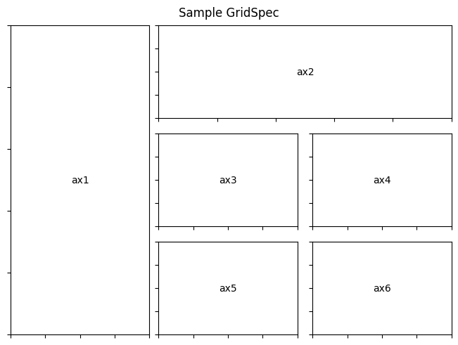
If you encounter it for the first time, it might seem confusing, and in all honesty, it’s just the bracket notation that is making this confusing. The declaration in this part simply states to create a grid specification of 3 rows and 3 columns in the fig object:

gs = GridSpec(nrows=3, ncols=3, figure=fig)

Which creates something like this behind the scenes:

By now you can see in this sample grid how the output was formed but reading the code, it seems so gibberish to undersaend.

The Syntax of Bracket Notation

By using the bracket notation, you first need to understand that its format is:

[rows, columns]

In any Python library, at least in the data science stack, this is the notation being used. I am not fond of this style, and I avoid it as much as possible because it is not easily readable. Additionally, having a good Python foundation is required to understand this bracket notation, which I hope this writing will help elucidate.

By avoiding the bracket notation, I would end up with something like this:

ax1 = fig.add_subplot(gs.new_subplotspec((0, 0), rowspan=3, colspan=1))
ax2 = fig.add_subplot(gs.new_subplotspec((0, 1), rowspan=1, colspan=2))
ax3 = fig.add_subplot(gs.new_subplotspec((1, 1), rowspan=1, colspan=1))
ax4 = fig.add_subplot(gs.new_subplotspec((1, 2), rowspan=1, colspan=1))
ax5 = fig.add_subplot(gs.new_subplotspec((2, 1), rowspan=1, colspan=1))
ax6 = fig.add_subplot(gs.new_subplotspec((2, 2), rowspan=1, colspan=1))

However, you won’t easily find this in the documentation. You still need to visit the GridSpecBase to see the new_subplotspec method. Additionally, the sample charts in the documentation use the bracket notation, which is much more concise than the alternative above.

The Start-Stop-Step Notation

Upon scanning the bracket notations used, one declaration is vastly different than the others. The use of GridSpec in ax2 involves the use of three numbers in the column specification.

The declaration of 1:3:1 means that start at 1, stop at 3, and add increments by 1. Another confusing aspect here is that the stop value is excluded. Therefore, 1:3 means from 1 to 2, excluding 3.

The use of 1:3:1 could be reduced to 1:3. The default value of 1 is always implied when you omit the step value:

ax2 = fig.add_subplot(gs[0, 1:3])

Normally, I would write it as 1:3, but using the complete notation makes it easier to understand.

The Counting System

In Python, the counting starts from 0.

Technically it is not “counting”, but rather the positions of data (index) start at 0, so in a list with 3 elements, you count it as 0, 1, 2.

This is known as zero-based indexing, a jargon that may already be familiar to those with a CS background, but not so for people like me.

Bringing Everything Together

With all these concepts in place, you already have the prerequisites to understand all of the Axes declarations that make the output the way it is.

ax1 = fig.add_subplot(gs[:, 0])
ax2 = fig.add_subplot(gs[0, 1:3:1])
ax3 = fig.add_subplot(gs[1, 1])
ax4 = fig.add_subplot(gs[1, 2])
ax5 = fig.add_subplot(gs[2, 1])
ax6 = fig.add_subplot(gs[2, 2])

Now, this is how most people interpret the bracket notation, which is certainly correct. However, the numerical values in the notation are mismatched with their associated descriptions.

The best approach to this is to apply the counting system from 0. Therefore, we should count the first position as 0, the second as 1, and so on.

All of these concepts can be encapsulated under indexing, but it is so CS-heavy that you have to know the concepts of indexes, data types, etc., and all the conventions that go with it in the Python language. This writing takes a more practical route; I introduced some of the indexing concepts that are directly relevant to the GridSpec usage. Here is the summary of those key concepts, ordered by importance:

• The counting/indexing in Python starts from 0.
• The bracket notation in Python follows the [rows, columns] syntax.
• The notation start:stop:step in Python is primarily used to obtain a subset of data.